
Over the past decade, we’ve seen diminishing importance of traditional statistics in data science. It used to be the case that statisticians would spend their time worrying about model specification and performing parameter estimation, but the advent of large datasets brought an emphasis on nonparametric models, out-of-sample validation, and the engineering work required to perform these tasks at scale.
This distinction was famously captured in Michael Hochster’s data scientist classification. To paraphrase,
Type A Data Scientist: A is for Analysis. They’re typically experts in topics taught in statistics departments, like experimental design, forecasting, modeling, and statistical inference, as well as the practical details of working with data, like data cleaning, methods for dealing with large data sets, visualization, and domain knowledge.
Type B Data Scientist: The B is for Build. They’re mainly interested in using data “in production”, building models which interact with users, and often serving recommendations. Many of their core competencies are shared with software engineers.
With the introduction of scikit-learn and PyTorch, data scientists can often train complicated models while understanding very little about how they work. Of course, since the release of ChatGPT and OpenAI’s API, the day-to-day work of the many applied ML researchers building LLM applications has moved even further away from traditional statistics.
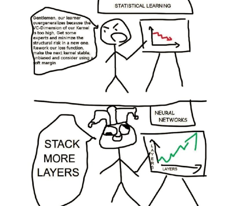
On a whole, the balance has shifted heavily towards Type B data scientists, and it’s hard to overstate the magnitude of the successes of deep learning: flexible models trained on massive datasets can capture behavior far more complicated than traditional statistics can. For good reasons, as expressed in this classic meme, the vibe since the late 2010’s has been “stack more layers”.
To be sure, producing (and consuming) cutting edge ML research requires a lot of technical ability. As anybody who’s tried to read papers promoting new neural net architectures or interpretability techniques knows, the rationales behind research directions are often expressed in dense mathematical prose. Machine learning is statistical learning, and when one technique works better than another, it’s fundamentally for mathematical reasons. Still, there’s a widespread attitude among practitioners that it’s enough to know how to code up architectures in PyTorch and correct obscure bugs, and that the math is someone else’s problem.
We at Hop put machine learning models into production, and we’re here to tell you that the math isn’t someone else’s problem. This post is the first in a series in which we highlight the ways that statistics creeps back into machine learning practice.
Vignette 1: Assessing third-party datasets to augment first-party data
One of our clients is a company that sells insurance to (in effect) small business owners, against risks related to transactions with customers. Often, little is known about these customers before transactions take place. Our team was responsible for estimating these risks.
Risk estimation for insurance is a standard application of machine learning, but three things complicated what would otherwise have been a textbook problem:
The target for our classification model was a class of rare events – less than 1% of transactions.
The small businesses were the ultimate consumers of our model outputs, and they were interested in risks associated with potential transactions relative to their usual distribution of transactions, rather than relative to all transactions insured by our client.
Information about customers was noisy and incomplete.
If any one of these three had been false, achieving the level of performance required by the business process would have been straightforward with the data we had. But under the circumstances, we needed more information about the customers, so we turned to third-party data to augment our first-party data.
The market for third-party data on individuals is large, illiquid, and opaque – in a first pass, we came across >100 datasets containing potentially relevant information, but few visible factors differentiated them from each other. This is a common position for purchasers of third-party data to be in, and the standard process for navigating it is to sign test contracts with vendors for access to limited amounts of data, continuing on to the purchase of full access to datasets if they’re deemed sufficiently valuable.
The key question:
How much data did we need in order to determine whether a dataset is worth purchasing?
If we tested a third-party dataset on too little data, we wouldn’t have enough statistical power to reliably detect real model performance improvements. But how little is too little? If even a hundred million records wouldn’t be enough, attempting to quantify the value of a dataset would have been a fool’s errand.
This turns out to be an experiment design problem related to the sort of A/B test sample size calculations that analytically oriented data scientists commonly perform¹. Under reasonable assumptions, minimum detectable effect size is given by the equation
$$\delta = \left(t_{\alpha/2}+t_\beta\right)\sigma\sqrt{2/n}$$
In our case, $\delta$ represented the improvement in model performance metric needed to justify purchase of a dataset, $\sigma$ the variance of the improvement in model performance², and $n$ the number of cross-validation splits we trained on³. The variables $t_{\alpha/2}$ and $t_{\beta}$ are the $t$-statistics associated with the significance level and power. The variable most directly impacted by the size of our test dataset was $\sigma$: with a larger dataset, model performance varies less from training run to training run, and smaller $\sigma$ allows detection of smaller effect sizes with better precision.
So far so good, but for ML models, larger datasets also come with changes in model performance, and potentially also changes in the extent to which new features improve model performance. Without accounting for these changes, our estimates for $\delta$ and $\sigma$ would be biased – so we modeled this bias.
We could measure improvements in model performance associated with the addition of third-party data on a small dataset, and we wanted to extrapolate those to improvements in performance associated with the addition of third-party data at our full dataset size.
We didn’t have access to third-party data at our full dataset size, of course, but what we could do was ablate subsets of features in our first-party dataset, and observe how model performance improvements from reintroducing those feature sets behaved across the full range of dataset sizes.
In essence, we filled in this square, using information from traversing the solid lines to inform our estimates of the effect of traversing the dashed lines:

Miraculously, a simple linear model was a very good fit for the behavior of model performance at different dataset sizes and feature sets. For performance metrics $p_{i,j}$ achieved by our model, subscript $i$ denoting training on either a base or extended feature set and subscript $j$ denoting training on a large or small dataset, we found that across a wide selection of feature subsets and dataset sizes, we could predict model performance on large datasets with extended feature sets to a high degree of accuracy with the formula:
$$p_{extended,\,large}=p_{base,\,large}+c\left(p_{extended,\,small}-p_{base,\,small}\right)$$
where $c$ is a constant depending only on the sizes of the small and large datasets. We derived a similar relationship governing the variance in model performance improvements, leaving us with all the ingredients necessary to extrapolate model performance improvements across dataset scales.
With this model in hand, we were able to target a (reasonable!) dataset size that would allow us to confidently determine which datasets improved model performance enough to justify their cost. In the end, none of the initial few datasets we investigated added discernable value. If we hadn’t done this analysis, we would have been left wondering, “Should we have asked for more data?” Instead, we knew that either improvements to our model’s performance were too small to be worth the purchase, or that we had been exposed to one of the rare false negatives permitted by our experiment design.
In many ways, we got lucky, and – caveat emptor – if you try to replicate these exact techniques, you may not find your data so amenable. Your model’s performance may not vary as predictably under changes in dataset size and feature inclusion, or it may be that the effect sizes you’re interested in require a lot more data to reliably detect. But regardless of the business problem and the specific model in use, the question “How much is this dataset worth to me?” is a central question, and the sort that demands that ML practitioners not forget their statistics.
— Liban Mohamed-Schwoebel, ML Researcher @ Hop
¹ For more information about sample sizes and statistical power in the context of A/B tests for conversion rates, see Evan Miller’s calculator and discussion.
² An important detail here was comparing the change in model performance for models trained on the same dataset splits – a lot of variation in measured model performance is due to concordance between train and test sets. By looking at the difference between so-paired models, we were able to extract a large variance reduction.
³ To reiterate, this $n$ is not the same as the size of the dataset being trained on, as it would be for most A/B tests in data science. Since data appearing in cross-validation splits aren’t independent across trials, there are diminishing returns to increasing the number of splits; fitting this parameter was also important in our analysis.